Today you will get some experience examining seismic velocities with a forward modeling approach. Forward modeling is a "guess and check" process, where we assign the seismic velocities, predict a syntehtic seismogram, and then compare the synthetic with the real observed seismogram. How well our guess does at matching the observation tells us how to change the seismic velocities on our next guess, so one has to keep careful track of the guesses.
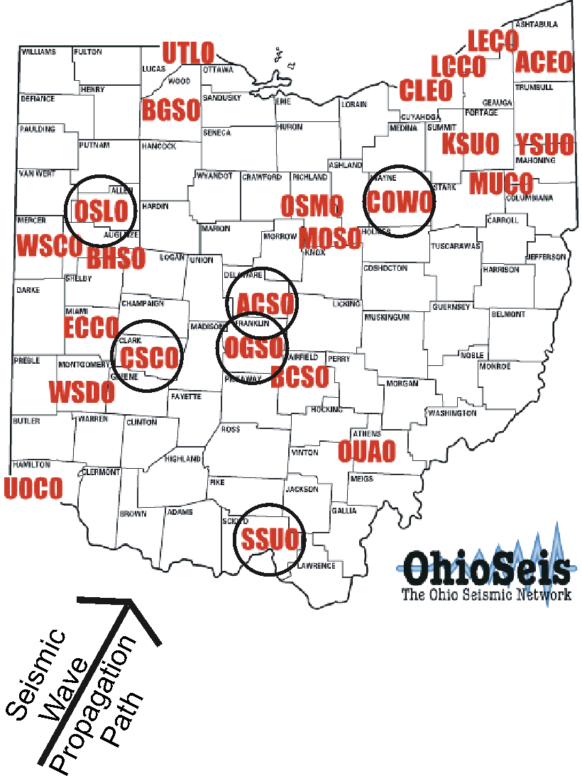
| The seismic data for today's activity comes from a seismic network here in Ohio that has been collecting data for over 10 years now. The data is primarily used for locating earthquakes that happen to occur in Ohio, but it can be used for other purposes as we will demonstrate today. This map shows the OhioSeis stations labeled in red, and I've circled stations which have recorded a distant large earthquake in southern Mexico that was recorded by the OhioSeis network. | 
|
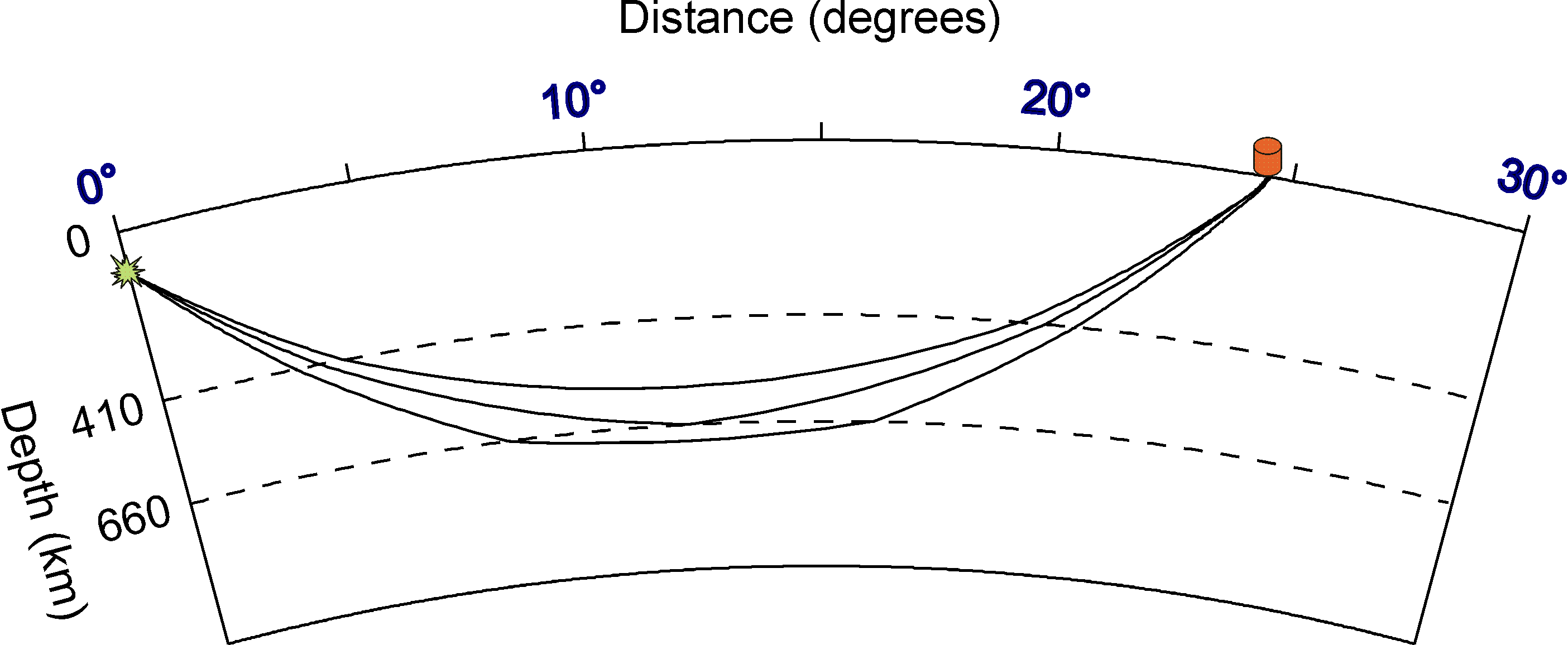
| Today we will use this data to look inside the Earth's mantle, at the transition zone between the upper and lower mantle. We can examine this region because there are velocity discontinuities at 410 and 660 km depth that define the top and bottom of the transition zone, and you should recall that seismic discontinuities generate triplications and multiple arrivals to analyze. This cross-section of the Earth shows the ray paths from the earthquake to one of the OhioSeis stations shows the multiple ray paths. | 
|
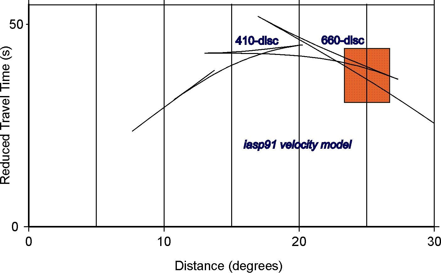
| This plot shows the corresponding travel time curve for this earthquake, and I've highlighted in red the region of the travel time curve since the locations of the OhioSeis stations correspond to those distances from the earthquake. As you go to larger distances in this red box, you can see there should be a move-out where the secondary arrivals become progressively later relative to the initial arrival. | 
|
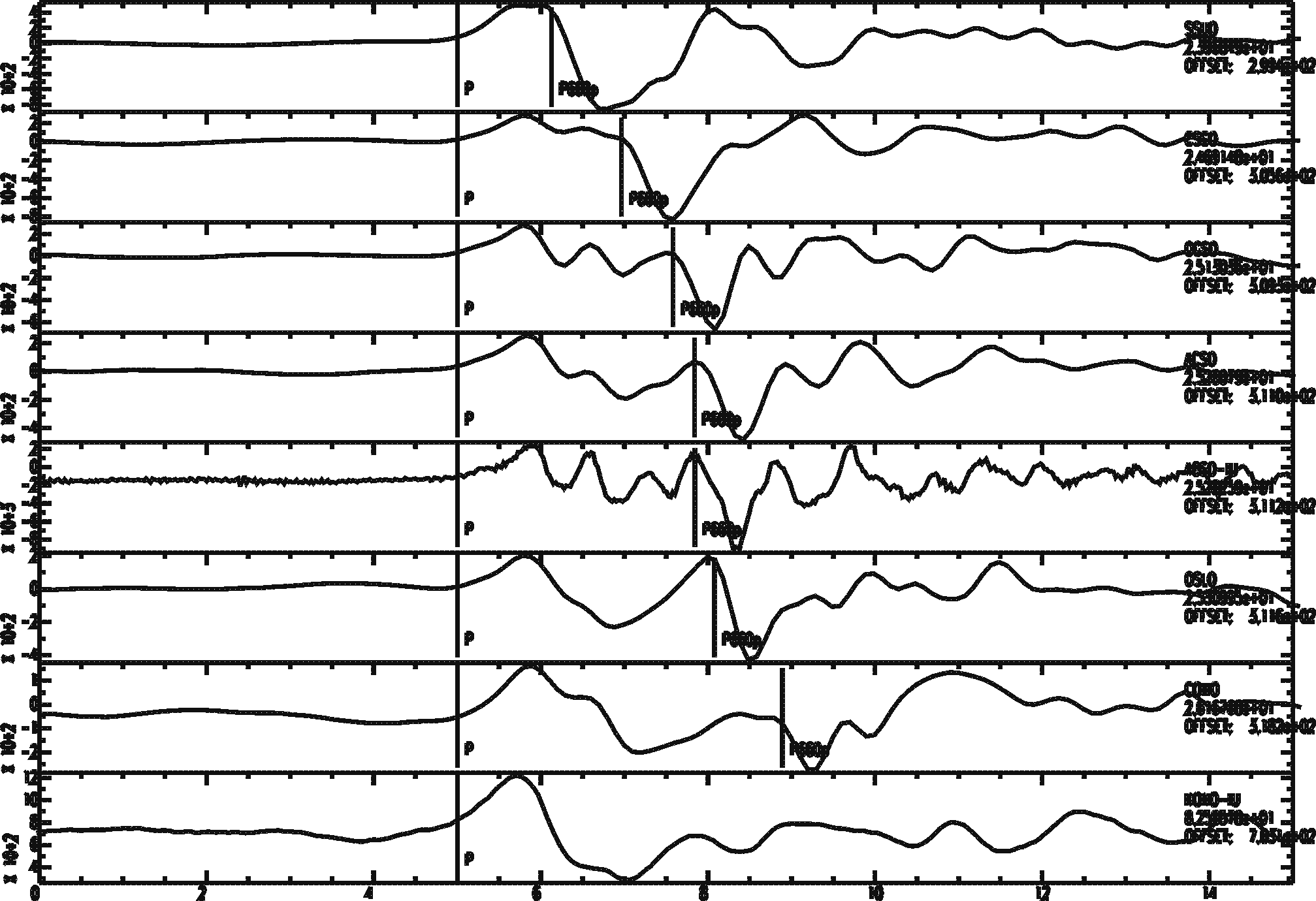
| The OhioSeis seismograms from this earthquake are shown below and they have been lined up with respect to their first arrival time (they have different absolute arrival times). They are plotted in order of increasing distance to show that yes, the secondary arrivals do become progressively later relative to the initial arrival. This means that the data is accurately representing the mantle transition zone. | 
|
Next we will try to match these multiple arrival observations with synthetic data to determine the seismic velocities in the mantle transition zone. To begin the processing part of this activity, let's login to the linux server with our VNC viewer, and then cd into the directory called
[username@linux ~] cd sac
[username@linux sac] mkdir synth
[username@linux sac] cd synth
[username@linux synth] cp /chiapas/mikeb/database/seismograms/ohioseis/*OSLO*.SAC .
It will also be important to copy a starting velocity model to this directory. We will copy an average earth velocity model to a file called
[username@linux synth] cp /chiapas/mikeb/wkbj/csh/iasp.mod test.mod
We will use a program called wkbj.csh to generate synthetic seismograms from this velocity model. This program requries a variety of command line information, so I will try to describe what it's asking for and then provide you with that information for this seismogram. The format is:.
wkbj.csh -ph seismic-phase -mod velocity-model -h event-depth -evt event-latitude event-longitude -sta station-latitude station-longitude -freq hi-or-lo-frequency -fps fault-plane-solution-(strike dip rake)
When we plug in all of the information you command should look like this:
[username@linux synth] wkbj.csh -ph P -mod test.mod -h 110 -evt 17.20 -95.22 -sta 40.729 -84.190 -freq lo -fps 161 27 -64
[username@linux synth] ls
You should notice with the ls command that
[username@linux synth] sac
SAC> r *.sac *.SAC
SAC> xlim t1 -10 10
SAC> p1
How do the two files compare? Similar, but not an exact match in the times of the two key arrivals (smaller first arrival, larger secondary arrival). We will do some forward modeling to try and get a better match. Go ahead and quit out of sac, and then I would suggest making a copy of the initial synthetic seismogram because it will help you to see your starting point. Then you can open up the test.mod file for editing.
SAC> quit
[username@linux synth] cp syn.P.lo.sac syn.P.lo.sac.start
[username@linux synth] emacs test.mod &
In the test.mod file, there are four lines to focus on during this forward modeling activity. The line for depth 409.95 represents the seismic properties above the transition zone, the line for depth 410.05 represents the properties at the top of the transition zone, depth 659.95 represents the properties at the bottom of the transition zone, and depth 660.05 represents the properties below the transition zone. You can adjust the values in teh second column (P wave velocities) and see how they affect you synthetic seismogram. I would only change them a few hundredths of a km/s at first, because that's all it takes to adjust the timing of the seimogram arrivals. I would also recommend starting your tests with the 409.95 line and working your way down.
Let's try adjusting the 409.95 line to be 9.08 instead of 9.03, save test.mod, and then run wkbj.csh again on the command line.
[username@linux synth] wkbj.csh -ph P -mod test.mod -h 110 -evt 17.20 -95.22 -sta 40.729 -84.190 -freq lo -fps 161 27 -64
[username@linux synth] sac
SAC> r *.sac *.SAC
SAC> xlim t1 -10 10
SAC> p1
Does this velocity produce better results than before? If you're not sure try reading in the
SAC> r more *start
SAC> p1
The velocity we changed to is worse, isn't it? It caused the arrivals to be earlier than they were before. That's because we increased the velocty from 9.03 to 9.08, and faster velocities cause earlier arrival times. We need to lower the velocity instead to get later arrival times that are closer to the observed times.
Spend some time varying the velocities on the four lines of test.mod I described above to try and get a good match between the arrival times in the observation and the synthetic seismogram. Describe your process in a file called synth.txt.
wkbj.csh information |
Script program to generate synthetic seismograms. |
brudzimr@muohio.edu, 6th November 2007