UNIX Tutorial Thirteen

13.1 Map of Plate Boundaries

For today's activity, we would like to make a map of plate boundaries. You have some experience making maps now, so I am going to ask you to do a little more of the command writing today. To help you out, I will give you some information about where the data files are, suggestions about how to organize the commands, and a new option to plot the line segments more clearly.

First, the data file for each of the three main types of plate boundaries can be found here:
/chiapas/mikeb/database/tect/PB2002/ridge.gmt
/chiapas/mikeb/database/tect/PB2002/trench.gmt
/chiapas/mikeb/database/tect/PB2002/transform.gmt

As in the past, you should copy these files to a new folder called act8. We will plot these line segments in Exercise 13.1 with psxy in a similar way to the exercise where we plotted the magnetic anomalies. You will need to specify the -JM and -R options with psxy, and you should make sure the -R ranges are large enough to see most of the world (I would recommend avoiding the latitudes above 70 North and below 70 South since the mercator projection does poorly with high latitudes). Recall that we also used the -M option for the multiple segments in the magnetic anomaly data file, since the plate boundary data files are also in this multiple segment format. In this case we have three different types of line segments to plot, so we'd like to distinguish them on our plot. We can do that if each data file is plotted with a different type of line.

13.2 Colored Line Segments

We can adjust the properties of the lines we plot using the -W option for psxy:

-W(line thickness)/(line color)

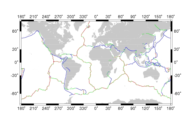
The line thickness is in points, with a thin line starting at 1, and the numbers increasing for thicker lines. The line color is a little more tricky, because we need to specify the color in Red/Green/Blue (RGB) values. Each of the RGB components can range from 0 to 255. For example, a nice clean red is 255/0/0, green is 0/255/0, and blue is 0/0/255. In our plate boundary plot I would recommend we plot each type of plate boundary with a different color (red, green, or blue). So in essence you will need to run psxy three times (once on each file, with a different color option) to plot each of the plate boundary types.

Exercise 13.1

Now I would like you to make a global map of the plate boundaries. There are two other suggestions I would make to help you accomplish this. First, you should use the pscoast command to plot continental areas first (see tutorial 11), so you can see where the plate boundaries actually are. The -D, -G, and -B commands can all be the same as in that tutorial, but you will want the -JM and -R options to be specifically for this plot (and the same as your psxy commands for this plot). Second, I would recommend you use a script file to organize all of your commands (see tutorial 6), since you will now need four commands to complete the map (1 pscoast, 3 psxy). You can call this script file platebound.csh, and the resulting plot file can be called platebound.ps. The finished plot should look something like this.

Since we will have 4 different GMT commands producing one plot, be careful to use the correct -K and -O options for your GMT commands, and use the >! characters to start a new file and >> to append to it.

Exercise 13.2

Once you have made a plot of global plate boundaries, I would like you to find and describe an area of the world for each of the types of plate boundary combinations introduced in class today (you should have 4 total locations):
(1) Ridge-Fault
(2) Fault-Trench (fault on concave side of trench)
(3) Fault-Trench (fault on convex side of trench)
(4) Ridge-Trench
Record your answers in a file called platebound.txt.

Exercise 13.3 (For next class period)

Once you have made a plot of global plate boundaries, I would like you to find and describe an area of the world for each of the types of plate boundary combinations introduced in class today (you should have 3 total locations):
(1) Ridge-Fault-Ridge
(2) Ridge-Fault-Trench
Since there are two types of case (2), describe whether the fault should be growing, or shrinking.
(3) Trench-Fault-Trench
Since there are three types of case (3), describe whether the fault should be growing, shrinking, or remaining the same size.
Record your answers in a file called platebound-3.txt.

Summary

brudzimr@muohio.edu, © 12th September 2006