UNIX Tutorial Ten

10.1 GMT Maps

In this tutorial we will begin to use the map making capabilities of GMT. In our previous tutorial we used the psxy command to make a simple X-Y plot of paleolatitudes versus age. Today we will use the same psxy command to make a map of magnetic anomalies with the Mercator projection. It is common for maps to be made with the Mercator projection as it produces a nice rectangular view, but it is important to remember that it does do a poor job of plotting areas near the poles. To produce a Mercator map with GMT, the -J option is the key for indicating that you want that type of plot. You will need to specify -JM for a Mercator map instead of the -JX option we used for the X-Y plot. You will still need a number at the end of the option (-JM6) to specify how big the X-axis should be in inches (the size of the Y-axis will be calculated for the Mercator projection).

To begin making a map, create a new directory called act5 in your groupwork directory. Then you can copy a version of the magnetic anomaly database over to your act5 directory. This file can be found at:
/chiapas/mikeb/database/tect/maglin/maglin.gmt

Take a look at the structure of this file (you can use a command like more) since it has already been formatted for use with psxy. You should notice that the first line of this file has a > character followed by a number and then successive lines have two numbers. The > character in the first line indicates that this contains header information and that it begins a new magnetic anomaly line segment. The following lines are longitude and latitude points of the magnetic anomaly segment. About ten lines down into the file, there is another header line indicating the next magnetic anomaly segment. The maglin.gmt file consists of nearly 6000 magnetic anomaly segments that have been mapped on the seafloor. We can plot line segments instead of symbols in psxy if we omit the -S option we used in our last tutorial. To tell psxy that we have multiple line segments we will use the -M option.

Since we have been looking at the paleolatitudes of India in our last few tutorials, we can now make a plot of the magnetic anomalies in the Indian Ocean. This will be an excellent comparison because it combines the continental-based paleomagnetism with the ocean-based paleomagnetism, which was a key development in the formation of the plate tectonic theory. If we want a map of that region, we need to select the range of longitude and latitude values that will represent that region, something like 40 to 90 longitude and -50 to -5 latitude. Since we will want to make some estimates of distance on this map, we should use the -B option to specify a relatively small tick interval like every 5 degrees. Here is the complete command that you can run to generate a map of the magnetic anomalies in this region:

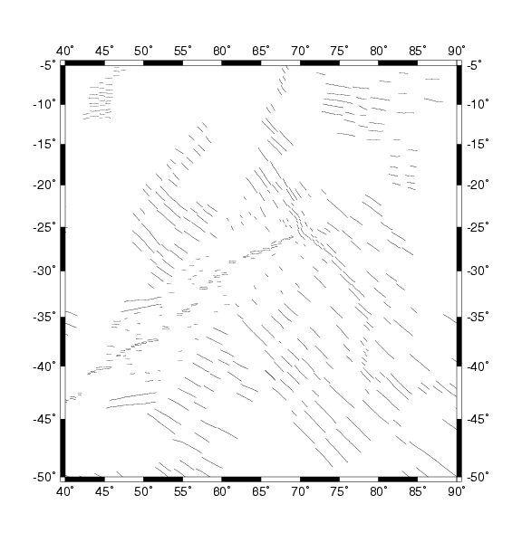
% psxy maglin.gmt -JM6 -R40/90/-50/-5 -M -B5/5 >! map.ps

Now take a look at the map you created (do you remember using the gv command as in our last tutorial?). It should have a series of line segments that look like this. You may be able to see the pattern of the mid-ocean ridge (Southest Indian Ridge), but it would certainly help if the magnetic anomalies were labeled in some way. Well it turns out that magnetic anomalies are often labeled by so-called "chron" numbers that correspond to prominent periods of normal (not reversed) polarity of the earth's magnetic field. The numbers get larger going back in time.

10.2 Plotting Text in GMT

There is a file we can use that has this chron information in it and you should copy this file to your act5 directory:
/chiapas/mikeb/database/tect/maglin/maglabel.txt

Take a look at the structure of this file as it has already been formatted for use with GMT. The format in this case is for the pstext command that is used for displaying text on a GMT plot. In this file, there are six columns of information about how to plot the text followed by the text to be plotted. A short label of each column is:

longitude latitude font-size font-type angle-to-rotate-text justification text

These is no need to go into the specifics of these values right now, because this is precisely the format expected by the pstext command so we can just specify this file as our input file. Otherwise pstext works in a very similar way to psxy:

pstext filename(s) options > psfile

We will still need to specify the -J and -R options just like we do for psxy. Since we want both the line segments and the text labels to appear on the same map we will need to have the psxy and pstext commands send their output to the same file (map-label.ps). GMT needs to know that you will be doing this so it can format the output correctly. The way to tell GMT about this is with the -K and -O options. -K means that more commands will add to the output file (I remember this by saying "more output is Koming"), and -O means that the output of the command should be Overlayed on top of the previous output. For our example, we will first use the psxy command to plot the line segments so it should have -K option and use the >! operator to generate a new output file, and second use the pstext command to plot the labels so it should have the -O option and the >> operator to append to the output file. Let's try it:

% psxy maglin.gmt -JM6 -R40/90/-50/-5 -M -B5/5 -K >! map-labels.ps
% pstext maglabel.txt -JM6 -R40/90/-50/-5 -O >> map-labels.ps

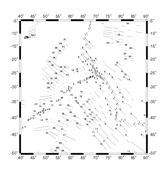
So what does this map look like? It should have the line segments with labels for the odd numbered magnetic anomalies that looks like this.

Exercise 10.1

First I would like you just to describe the patterns you can see in the magnetic anomalies. Open a new text file called patterns.txt and describe in words what the magnetic anomalies show. What does the mid-ocean ridge look like? Are there offsets in the magnetic anomalies? Are there areas that don't match neighboring regions? What do you think has caused some of these patterns?

Exercise 10.2

Now I would like you to calculate the half-spreading rate of the Southeast Indian Ridge using the method described in class: distance between anomalies / time between anomalies. First measure the approximate distance between chron 1 (0.4 Ma - Ma stands for million years old) and chron 5 (10 Ma). You can use the latitude scale on the Y-axis as your guide for distance and the fact that 1 degree roughly translates to 111 km. When you divide the distance by the time, it is useful to note that kilometers are 10⁶ millimeters and Ma are 10⁶ years, so your half-spreading rate should be in mm/yr. You should do the same calculation for the distance between chron 25 (59 Ma) and chron 31 (69 Ma). Store your results in a file called rates.txt including which rate is for which chrons.

Exercise 10.3

Lastly, I would like you to assess why the values calculated in Exercise 10.2 are different. What is different between those two time periods? You should also compare these estimates with the information stored in your age-paleolat.txt file from the last tutorial. In this case, you can calculate the rates of motion for the 0 to 20 Ma time frame and the 20 to 65 Ma time frame based on the changes in paleolatitude (remember degrees of latitude are about 111 km). Are the rates from the paleolatitude information larger or smaller than the rates from the magnetic anomalies? Why? Store your answers for this exercise in a file called comparison.txt.

Summary

brudzimr@muohio.edu, © 19th August 2006